シミュレーション105：数値積分によるダブルペンデュラムモデリング

Simulation 105 Double Pendulum Modeling with Numerical Integration

混沌系のモデリング

振り子は私たちが皆よく知っている古典物理学のシステムです。祖父時計やブランコの子供など、私たちは振り子の規則的で周期的な動きを見たことがあります。単一の振り子は古典物理学ではよく定義されていますが、ダブルペンデュラム（別のペンデュラムの先に取り付けられたペンデュラム）は文字通りの混沌です。本稿では、振り子に対する直感的な理解を基にして、ダブルペンデュラムの混沌をモデル化します。物理学は興味深く、数値計算手法は誰の武器にも欠かせないツールです。

この記事では、以下のことを学びます：

調和運動について学び、単一の振り子の挙動をモデル化する
混沌理論の基礎を学ぶ
ダブルペンデュラムの混沌的な挙動を数値的にモデル化する

調和運動と単一の振り子

単純調和運動

振り子の周期的な振動運動を調和運動と呼びます。調和運動は、システム内の運動が、逆方向に比例する復元力によってバランスされる場合に起こります。図2では、ばねに取り付けられた物体が重力によって引っ張られるが、これによってばねにエネルギーが入り、ばねが反発して物体を引き上げる様子が示されています。ばね系の隣には、物体の高さが円を描く位相線図があり、システムの規則的な運動がさらに説明されています。

調和運動は、減衰（ドラッグ力による振幅の減少）または駆動（外部力の追加による振幅の増加）される場合もありますが、これからは外部力が作用せずに振幅が無限に続く単純な調和運動の場合から始めます（減衰しない運動）。これは、小さな角度/低振幅で揺れる単一の振り子をモデル化するための良い近似です。この場合、以下の式（式1）で運動をモデル化することができます。

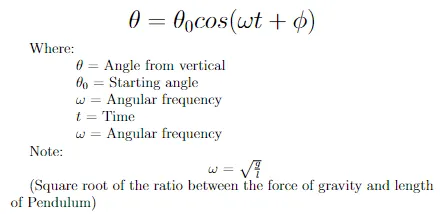
この関数を簡単にコードに入れて、時間の経過とともに単純な振り子をシミュレーションできます。

def simple_pendulum(theta_0, omega, t, phi):    theta = theta_0*np.cos(omega*t + phi)    return theta#parameters of our systemtheta_0 = np.radians(15) #degrees to radiansg = 9.8 #m/s^2l = 1.0 #momega = np.sqrt(g/l)phi = 0 #for small angletime_span = np.linspace(0,20,300) #simulate for 20s split into 300 time intervalstheta = []for t in time_span:    theta.append(simple_pendulum(theta_0, omega, t, phi))#Convert back to cartesian coordinatesx = l*np.sin(theta)y = -l*np.cos(theta) #negative to make sure the pendulum is facing down

ラグランジュ力学による完全な振り子運動

シンプルな小角度振り子は良いスタートですが、私たちはこれを超えて完全な振り子の運動をモデル化したいと考えています。小角度の近似を使用することはできなくなるため、最も適した方法はラグランジュ力学を使用して振り子をモデル化することです。これは、システム内の力ではなくエネルギーを見るための物理学の必須ツールです。私たちは、駆動力対復元力から運動エネルギー対ポテンシャルエネルギーへの視点を切り替えています。

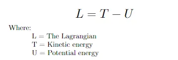
ラグランジュ関数は、式2で与えられる運動エネルギーとポテンシャルエネルギーの差です。

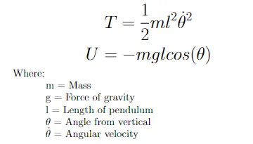
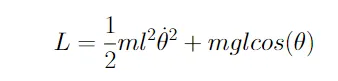
式3で与えられる振り子の運動エネルギーとポテンシャルエネルギーを代入すると、式4で示される振り子のラグランジュ関数が得られます。

振り子のラグランジュ関数を使用して、システムのエネルギーを記述します。シミュレーションを構築するためには、エネルギー参照から力指向の動的参照に戻るために、オイラー・ラグランジュ方程式を使用する必要があります。この方程式を使用することで、ラグランジュ関数を使用して振り子の角加速度を得ることができます。

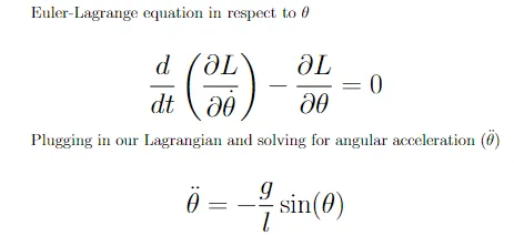
数学的な処理を経て、角加速度を得ることができます。これを使用して角速度と角度を取得する必要があります。これには数値積分が必要で、完全な振り子シミュレーションで説明されます。単一の振り子でも、非線形のダイナミクスにより、θを解くための解析的な解は存在せず、数値解が必要です。積分は非常にシンプルですが（しかし強力です）、角加速度を使用して角速度を更新し、角速度を前者の量に加え、これにいくつかの時間ステップを乗算してθを更新します。これにより、加速度/速度曲線の面積の近似値が得られます。時間ステップが小さいほど、近似値はより正確になります。

def full_pendulum(g,l,theta,theta_velocity, time_step):    #数値積分    theta_acceleration = -(g/l)*np.sin(theta) #加速度を取得    theta_velocity += time_step*theta_acceleration #加速度で速度を更新    theta += time_step*theta_velocity #角速度で角度を更新    return theta, theta_velocityg = 9.8 #m/s^2l = 1.0 #mtheta = [np.radians(90)] #初期角度theta_0theta_velocity = 0 #初期速度time_step = 20/300 #時間ステップを定義time_span = np.linspace(0,20,300) #20秒間を300の時間間隔に分割for t in time_span:    theta_new, theta_velocity = full_pendulum(g,l,theta[-1], theta_velocity, time_step)    theta.append(theta_new)#デカルト座標に戻すための変換 x = l*np.sin(theta)y = -l*np.cos(theta)

完全な振り子のシミュレーションを実施しましたが、これはまだ明確に定義されたシステムです。今度は、ダブル振り子の混沌に足を踏み入れる時です。

カオスと二重振り子

数学的な意味でのカオスとは、初期条件に非常に敏感なシステムを指します。システムの開始時にわずかな変化があるだけで、システムの進化によって大きく異なる振る舞いが生じます。これは二重振り子の運動を完璧に表しています。単振り子とは異なり、二重振り子は予測可能な振る舞いを示さず、わずかな開始角度の変化でも大きく異なる方法で進化します。

二重振り子の運動をモデル化するために、前回と同じラグランジュアプローチを使用します（詳細な導出はこちらを参照してください）。

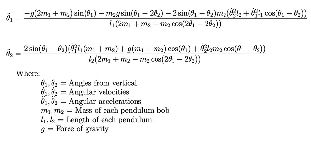
また、この方程式をコードに実装し、θを求める際には前回と同じ数値積分手法も使用します。

#θ1の加速度を取得するdef theta1_acceleration(m1,m2,l1,l2,theta1,theta2,theta1_velocity,theta2_velocity,g):    mass1 = -g*(2*m1 + m2)*np.sin(theta1)    mass2 = -m2*g*np.sin(theta1 - 2*theta2)    interaction = -2*np.sin(theta1 - theta2)*m2*np.cos(theta2_velocity**2*l2 + theta1_velocity**2*l1*np.cos(theta1 - theta2))    normalization = l1*(2*m1 + m2 - m2*np.cos(2*theta1 - 2*theta2))        theta1_ddot = (mass1 + mass2 + interaction)/normalization        return theta1_ddot#θ2の加速度を取得するdef theta2_acceleration(m1,m2,l1,l2,theta1,theta2,theta1_velocity,theta2_velocity,g):    system = 2*np.sin(theta1 - theta2)*(theta1_velocity**2*l1*(m1 + m2) + g*(m1 + m2)*np.cos(theta1) + theta2_velocity**2*l2*m2*np.cos(theta1 - theta2))    normalization = l1*(2*m1 + m2 - m2*np.cos(2*theta1 - 2*theta2))        theta2_ddot = system/normalization    return theta2_ddot#θ1を更新するdef theta1_update(m1,m2,l1,l2,theta1,theta2,theta1_velocity,theta2_velocity,g,time_step):    #数値積分    theta1_velocity += time_step*theta1_acceleration(m1,m2,l1,l2,theta1,theta2,theta1_velocity,theta2_velocity,g)    theta1 += time_step*theta1_velocity    return theta1, theta1_velocity#θ2を更新するdef theta2_update(m1,m2,l1,l2,theta1,theta2,theta1_velocity,theta2_velocity,g,time_step):    #数値積分    theta2_velocity += time_step*theta2_acceleration(m1,m2,l1,l2,theta1,theta2,theta1_velocity,theta2_velocity,g)    theta2 += time_step*theta2_velocity    return theta2, theta2_velocity#二重振り子の全体を実行するdef double_pendulum(m1,m2,l1,l2,theta1,theta2,theta1_velocity,theta2_velocity,g,time_step,time_span):    theta1_list = [theta1]    theta2_list = [theta2]        for t in time_span:        theta1, theta1_velocity = theta1_update(m1,m2,l1,l2,theta1,theta2,theta1_velocity,theta2_velocity,g,time_step)        theta2, theta2_velocity = theta2_update(m1,m2,l1,l2,theta1,theta2,theta1_velocity,theta2_velocity,g,time_step)        theta1_list.append(theta1)        theta2_list.append(theta2)        x1 = l1*np.sin(theta1_list) #振り子1のx座標    y1 = -l1*np.cos(theta1_list) #振り子1のy座標    x2 = l1*np.sin(theta1_list) + l2*np.sin(theta2_list) #振り子2のx座標    y2 = -l1*np.cos(theta1_list) - l2*np.cos(theta2_list) #振り子2のy座標        return x1,y1,x2,y2

#システムパラメータを定義するg = 9.8 #m/s^2m1 = 1 #kgm2 = 1 #kgl1 = 1 #ml2 = 1 #mtheta1 = np.radians(90)theta2 = np.radians(45)theta1_velocity = 0 #m/stheta2_velocity = 0 #m/stheta1_list = [theta1]theta2_list = [theta2]time_step = 20/300time_span = np.linspace(0,20,300)x1,y1,x2,y2 = double_pendulum(m1,m2,l1,l2,theta1,theta2,theta1_velocity,theta2_velocity,g,time_step,time_span)

やっとできました！二重振り子を成功裏にモデル化しましたが、今度は混沌を観察する時です。最終的なシミュレーションでは、わずかに異なる初期条件を持つ2つの二重振り子を使用します。1つの振り子ではθ1を90度に設定し、もう1つの振り子ではθ1を91度に設定します。どうなるか見てみましょう。

両方の振り子が似た軌道から始まりますが、すぐに分岐します。これが私たちが混沌と言う意味です。わずかな角度の1度の違いでも、大きく異なる最終的な振る舞いになります。

結論

この記事では、振り子の運動とそのモデリング方法について学びました。最も単純な調和運動モデルから始めて、複雑でカオスな二重振り子まで構築しました。途中でラグランジアン、カオス、数値積分について学びました。

二重振り子は、混沌系の最も単純な例です。これらの系は、人口動態、気候、さらにはビリヤードなど、私たちの世界中に存在しています。二重振り子から学んだ教訓を、混沌的なシステムに遭遇したときにいつでも適用することができます。

重要なポイント

混沌系は初期条件に非常に敏感であり、わずかな変化でも大きく異なる経路で進化します。
システムに取り組む際、特に混沌系に取り組む際に、より扱いやすい視点はありますか？（力の基準フレームからエネルギーの基準フレームなど）
システムが複雑になりすぎると、数値的な解を実装する必要があります。これらの解は簡単ですが強力であり、実際の振る舞いに良い近似を提供します。

参考文献

この記事で使用されているすべての図は、著者によって作成されたものまたはMath Imagesから提供されたもので、GNU Free Documentation License 1.2のもとで公開されています。

すべて-はい、すべては調和振動子です

物理学の学部生は、宇宙が調和振動子でできていると冗談を言うかもしれませんが、それはそれほど間違っていません。

www.wired.com

Classical Mechanics, John Taylor https://neuroself.files.wordpress.com/2020/09/taylor-2005-classical-mechanics.pdf

フルコード

単振り子

def makeGif(x,y,name):    !mkdir frames        counter=0    images = []    for i in range(0,len(x)):        plt.figure(figsize = (6,6))        plt.plot([0,x[i]],[0,y[i]], "o-", color = "b", markersize = 7, linewidth=.7 )        plt.title("Pendulum")        plt.xlim(-1.1,1.1)        plt.ylim(-1.1,1.1)        plt.savefig("frames/" + str(counter)+ ".png")        images.append(imageio.imread("frames/" + str(counter)+ ".png"))        counter += 1        plt.close()    imageio.mimsave(name, images)    !rm -r framesdef simple_pendulum(theta_0, omega, t, phi):    theta = theta_0*np.cos(omega*t + phi)    return theta#parameters of our systemtheta_0 = np.radians(15) #degrees to radiansg = 9.8 #m/s^2l = 1.0 #momega = np.sqrt(g/l)phi = 0 #for small angletime_span = np.linspace(0,20,300) #simulate for 20s split into 300 time intervalstheta = []for t in time_span:    theta.append(simple_pendulum(theta_0, omega, t, phi))x = l*np.sin(theta)y = -l*np.cos(theta) #negative to make sure the pendulum is facing down

振り子

def full_pendulum(g,l,theta,theta_velocity, time_step):    theta_acceleration = -(g/l)*np.sin(theta)    theta_velocity += time_step*theta_acceleration    theta += time_step*theta_velocity    return theta, theta_velocityg = 9.8 #m/s^2l = 1.0 #mtheta = [np.radians(90)] #theta_0theta_velocity = 0time_step = 20/300time_span = np.linspace(0,20,300) #20秒間を300の時間間隔でシミュレートするfor t in time_span:    theta_new, theta_velocity = full_pendulum(g,l,theta[-1], theta_velocity, time_step)    theta.append(theta_new)#デカルト座標に変換する x = l*np.sin(theta)y = -l*np.cos(theta)#単振り子と同じ関数を使用してGIFを作成するmakeGif(x,y,"pendulum.gif")

二重振り子

def theta1_acceleration(m1,m2,l1,l2,theta1,theta2,theta1_velocity,theta2_velocity,g):    mass1 = -g*(2*m1 + m2)*np.sin(theta1)    mass2 = -m2*g*np.sin(theta1 - 2*theta2)    interaction = -2*np.sin(theta1 - theta2)*m2*np.cos(theta2_velocity**2*l2 + theta1_velocity**2*l1*np.cos(theta1 - theta2))    normalization = l1*(2*m1 + m2 - m2*np.cos(2*theta1 - 2*theta2))        theta1_ddot = (mass1 + mass2 + interaction)/normalization        return theta1_ddotdef theta2_acceleration(m1,m2,l1,l2,theta1,theta2,theta1_velocity,theta2_velocity,g):    system = 2*np.sin(theta1 - theta2)*(theta1_velocity**2*l1*(m1 + m2) + g*(m1 + m2)*np.cos(theta1) + theta2_velocity**2*l2*m2*np.cos(theta1 - theta2))    normalization = l1*(2*m1 + m2 - m2*np.cos(2*theta1 - 2*theta2))        theta2_ddot = system/normalization    return theta2_ddotdef theta1_update(m1,m2,l1,l2,theta1,theta2,theta1_velocity,theta2_velocity,g,time_step):        theta1_velocity += time_step*theta1_acceleration(m1,m2,l1,l2,theta1,theta2,theta1_velocity,theta2_velocity,g)    theta1 += time_step*theta1_velocity    return theta1, theta1_velocitydef theta2_update(m1,m2,l1,l2,theta1,theta2,theta1_velocity,theta2_velocity,g,time_step):        theta2_velocity += time_step*theta2_acceleration(m1,m2,l1,l2,theta1,theta2,theta1_velocity,theta2_velocity,g)    theta2 += time_step*theta2_velocity    return theta2, theta2_velocitydef double_pendulum(m1,m2,l1,l2,theta1,theta2,theta1_velocity,theta2_velocity,g,time_step,time_span):    theta1_list = [theta1]    theta2_list = [theta2]        for t in time_span:        theta1, theta1_velocity = theta1_update(m1,m2,l1,l2,theta1,theta2,theta1_velocity,theta2_velocity,g,time_step)        theta2, theta2_velocity = theta2_update(m1,m2,l1,l2,theta1,theta2,theta1_velocity,theta2_velocity,g,time_step)        theta1_list.append(theta1)        theta2_list.append(theta2)        x1 = l1*np.sin(theta1_list)    y1 = -l1*np.cos(theta1_list)    x2 = l1*np.sin(theta1_list) + l2*np.sin(theta2_list)    y2 = -l1*np.cos(theta1_list) - l2*np.cos(theta2_list)        return x1,y1,x2,y2

#系統パラメータの定義、二重振り子を実行するg = 9.8 #m/s^2m1 = 1 #kgm2 = 1 #kgl1 = 1 #ml2 = 1 #mtheta1 = np.radians(90)theta2 = np.radians(45)theta1_velocity = 0 #m/stheta2_velocity = 0 #m/stheta1_list = [theta1]theta2_list = [theta2]time_step = 20/300time_span = np.linspace(0,20,300)for t in time_span:    theta1, theta1_velocity = theta1_update(m1,m2,l1,l2,theta1,theta2,theta1_velocity,theta2_velocity,g,time_step)    theta2, theta2_velocity = theta2_update(m1,m2,l1,l2,theta1,theta2,theta1_velocity,theta2_velocity,g,time_step)        theta1_list.append(theta1)    theta2_list.append(theta2)    x1 = l1*np.sin(theta1_list)y1 = -l1*np.cos(theta1_list)x2 = l1*np.sin(theta1_list) + l2*np.sin(theta2_list)y2 = -l1*np.cos(theta1_list) - l2*np.cos(theta2_list)

#GIFを作成するためにフォルダを作成するmkdir frames    counter=0images = []for i in range(0,len(x1)):    plt.figure(figsize = (6,6))    plt.figure(figsize = (6,6))    plt.plot([0,x1[i]],[0,y1[i]], "o-", color = "b", markersize = 7, linewidth=.7 )    plt.plot([x1[i],x2[i]],[y1[i],y2[i]], "o-", color = "b", markersize = 7, linewidth=.7 )    plt.title("二重振り子")    plt.xlim(-2.1,2.1)    plt.ylim(-2.1,2.1)    plt.savefig("frames/" + str(counter)+ ".png")    images.append(imageio.imread("frames/" + str(counter)+ ".png"))    counter += 1    plt.close()imageio.mimsave("double_pendulum.gif", images)!rm -r frames

We will continue to update VoAGI; if you have any questions or suggestions, please contact us!

Classical MechanicsComputationNumerical MethodsPhysicsSimulation

Was this article helpful?

93 out of 132 found this helpful