「生データから洗練されたデータへ：データの前処理を通じた旅 – パート1」

From raw data to refined data Journey through data preprocessing - Part 1

時には、機械学習のタスクに適した形式で提供されないデータがあります。そのため、データを処理して所望の形式に変換する必要があります。

元データにはさまざまな問題があります。問題の性質に応じて、適切な方法を使用して対処する必要があります。

いくつかの方法とそのコード実装について見てみましょう。

平均除去と分散スケーリング（標準化）

• 「ソフトウェア開発におけるAIの活用：ソリューション戦略と実装」
• 「Med-PaLM Multimodal（Med-PaLM M）をご紹介します：柔軟にエンコードし、解釈するバイオメディカルデータの大規模なマルチモーダル生成モデル」
• 「BI-LSTMを用いた次の単語予測のマスタリング：包括的なガイド」

Scikit-Learnの推定器（推定器とは、機械学習モデルのトレーニングに使用されるScikit-Learnのクラスを指します）は、標準的な正規分布のデータ、つまり平均がゼロで分散が1のガウス分布で最も効果的に動作するように調整されています。

元データは常にガウス分布ではないため、このデータでトレーニングされたモデルは最適な結果を得られない場合があります。この問題の解決策は、標準化操作です。

標準化は以下の式を使用して行われます：

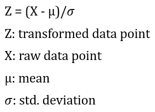
まず、列ごとに平均と標準偏差を計算します。次に、その列のすべてのデータ点から平均を引きます。最後に、引き算の結果を標準偏差で割ります。

この方法をコードで実装してみましょう。

デモンストレーションのために、有名な「Tips」データセットを使用しましょう。「Tips」データセットは、総額、顧客の性別、曜日、時間帯などのさまざまな要素に基づいてウェイターが受け取るチップを予測するために使用されます。

## 必要なライブラリのインポートimport warningswarnings.filterwarnings('ignore')import numpy as npimport pandas as pdimport matplotlib.pyplot as pltimport seaborn as sns%matplotlib inline

## データの読み込みdf = pd.read_csv('https://raw.githubusercontent.com/mwaskom/seaborn-data/master/tips.csv')## データの最初のいくつかの行を確認するdf.head()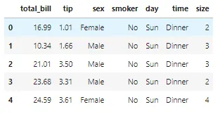

まず、独立変数から従属変数である「total_bill」を分離する必要があります。その後、データをトレーニングセットとテストセットに分割する必要があります。

## 必要なメソッドのインポートfrom sklearn.model_selection import train_test_split## 従属変数と独立変数の分離X, y = df.drop('total_bill', axis=1), df['total_bill']## トレーニングデータとテストデータの分離X_train, X_test, y_train, y_test = train_test_split(X, y, random_state=42)

「tip」列に対して標準スケーリングを実行しましょう。

from sklearn.preprocessing import StandardScaler## 列の平均と標準偏差を計算するscaler = StandardScaler().fit(np.array(X_train['tip']).reshape(-1,1))## 計算された平均と標準偏差を使用してデータを変換するtips_transformed = scaler.transform(np.array(X_test['tip']).reshape(-1,1))tips_transformed[:10]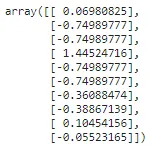

「reshape」メソッドは、fitおよびtransformメソッドには2次元配列が必要なため、1次元配列を2次元配列に変換するために使用されます。

範囲にスケーリングする（MinMaxScalerおよびMaxAbsScaler）

これは標準化の別のアプローチで、特徴量を最小値と最大値の間、通常は0から1の間、または各特徴量の最大絶対値が単位サイズにスケーリングされるようにスケーリングします。

MinMaxScalerを使用してデータを「min」と「max」の値の間にスケーリングする場合、以下の式が使用されます：

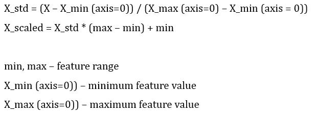
MinMaxScaler:

from sklearn.preprocessing import MinMaxScaler## 列の平均値と標準偏差を計算するmm_scaler = MinMaxScaler().fit(np.array(X_train['tip']).reshape(-1,1))## 計算された平均値と標準偏差を用いてデータを変換するtips_transformed = mm_scaler.transform(np.array(X_test['tip']).reshape(-1,1))tips_transformed[:10]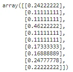

MaxAbsScalerは同様の方法で動作しますが、各値が範囲[-1, 1]に収まるようにデータをスケーリングします。これは、各特徴量ごとに最大値で除算することによって行われます。

データの中心化はデータのスパース性を破壊し、一般的には適切ではありません。ただし、特徴量が異なるスケールである場合は、スパースな入力をスケーリングすることは合理的です。MaxAbsScalerは、スパースデータのスケーリングのために特に設計されており、推奨される方法です。

MaxAbsScaler:

from sklearn.preprocessing import MaxAbsScaler## 列の平均値と標準偏差を計算するma_scaler = MaxAbsScaler().fit(np.array(X_train['tip']).reshape(-1,1))## 計算された平均値と標準偏差を用いてデータを変換するtips_transformed = ma_scaler.transform(np.array(X_test['tip']).reshape(-1,1))tips_transformed[:10]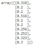

外れ値を含むデータのスケーリング（RobustScaler）

データに外れ値が多く含まれている場合、平均値と標準偏差の値は歪んでしまう可能性があります。この場合、外れ値のあるデータに対して平均値と標準偏差を使用すると、データの中心やデータの範囲を正しく表現できません。

この問題を回避するために、より頑健な推定値を使用するRobustScalerを使用することができます。これにより、データの中心と範囲がより正確に表現されます。

from sklearn.preprocessing import RobustScaler## 列の平均値と標準偏差を計算するr_scaler = RobustScaler().fit(np.array(X_train['tip']).reshape(-1,1))## 計算された平均値と標準偏差を用いてデータを変換するtips_transformed = r_scaler.transform(np.array(X_test['tip']).reshape(-1,1))tips_transformed[:10]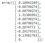

一様分布へのマッピング（QuantileTransformer）

QuantileTransformerは、データを0から1の範囲の一様分布にマッピングするために使用できます。

from sklearn.preprocessing import QuantileTransformerq_transformer = QuantileTransformer().fit(np.array(X_train['tip']).reshape(-1,1))xtrain_transformed = q_transformer.transform(np.array(X_train['tip']).reshape(-1,1))

さて、変換前と変換後の’tip’列を可視化しましょう。

dataframe = pd.DataFrame()dataframe['tips_given'] = X_train['tip']dataframe['tips_uniformDist'] = xtrain_transformedsns.set_style('darkgrid')plt.figure(figsize=(10,5))for index, feature in enumerate(dataframe.columns):    plt.subplot(1,2,index+1)    sns.distplot(dataframe[feature],kde=True, color='b')    plt.xlabel(feature)    plt.ylabel('distribution')    plt.title(f"{feature} distribution")plt.tight_layout()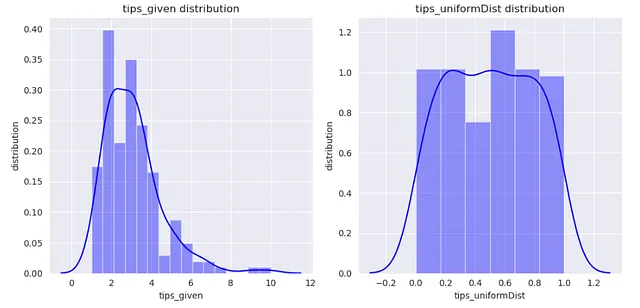

ガウス分布へのマッピング（PowerTransformer）

PowerTransformerを使用してデータをガウス分布にできるだけ近い分布にマッピングすることができます。

この変換を行うために使用できる2つの方法があります。

1. Box-cox変換
2. Yeo-Johnson変換

ボックスコックス変換は、正のデータにのみ適用できることに注意してください。

ボックスコックス変換：

from sklearn.preprocessing import PowerTransformer
p_transformer = PowerTransformer(method='box-cox').fit(np.array(X_train['tip']).reshape(-1,1))
xtrain_transformed = p_transformer.transform(np.array(X_train['tip']).reshape(-1,1))

dataframe = pd.DataFrame()
dataframe['tips_given'] = X_train['tip']
dataframe['tips_NormalDist'] = xtrain_transformed

sns.set_style('darkgrid')
plt.figure(figsize=(10,5))
for index, feature in enumerate(dataframe.columns):
    plt.subplot(1,2,index+1)
    sns.distplot(dataframe[feature],kde=True, color='y')
    plt.xlabel(feature)
    plt.ylabel('distribution')
    plt.title(f"{feature}の分布")
plt.tight_layout()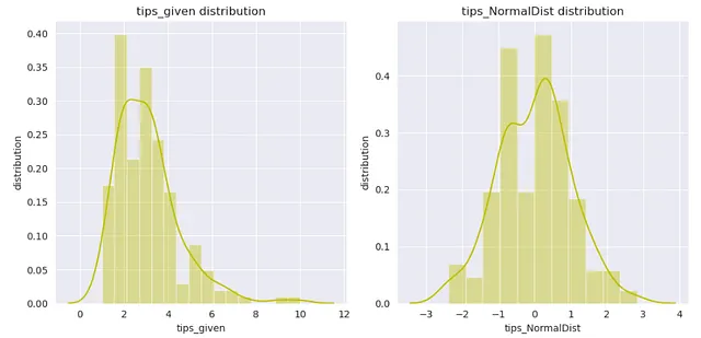

イェオジョンソン変換：

from sklearn.preprocessing import PowerTransformer
p_transformer = PowerTransformer(method='yeo-johnson').fit(np.array(X_train['tip']).reshape(-1,1))
xtrain_transformed = p_transformer.transform(np.array(X_train['tip']).reshape(-1,1))

dataframe = pd.DataFrame()
dataframe['tips_given'] = X_train['tip']
dataframe['tips_NormalDist'] = xtrain_transformed

sns.set_style('darkgrid')
plt.figure(figsize=(10,5))
for index, feature in enumerate(dataframe.columns):
    plt.subplot(1,2,index+1)
    sns.distplot(dataframe[feature],kde=True, color='g')
    plt.xlabel(feature)
    plt.ylabel('distribution')
    plt.title(f"{feature}の分布")
plt.tight_layout()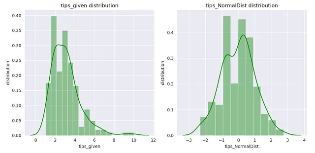

記事がお気に入りになると嬉しいです。記事についてのご意見があれば、お知らせください。また、この前処理シリーズの次の記事にもご期待ください。

連絡先：

LinkedIn

ウェブサイト

メール：[email protected]

素晴らしい一日をお過ごしください！

We will continue to update VoAGI; if you have any questions or suggestions, please contact us!